GOOGL 6成底仓 + 4成浮动仓 RSI 策略回测
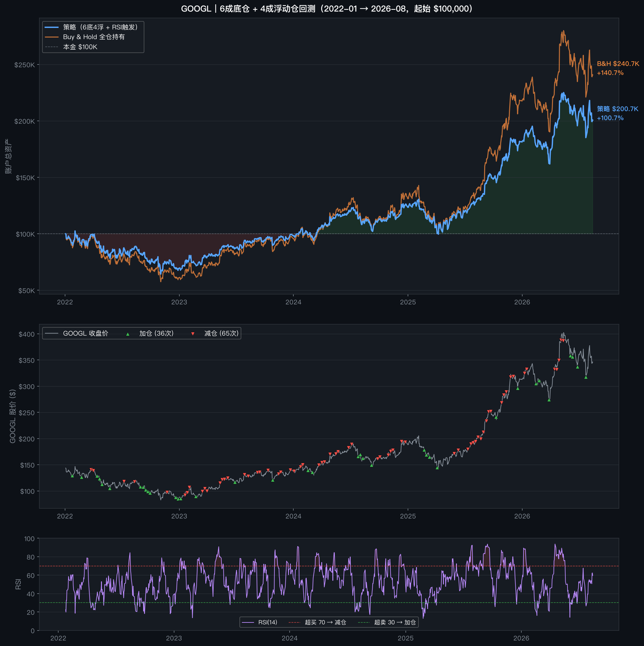
一句话结论:策略最终 +100.7%,Buy & Hold +140.7%。少亏了熊市 6 个点,也少赚了牛市 40 个点。拿回撤换踏空,在趋势股上是赔本买卖。
策略设计
| 参数 | 设定 |
|---|---|
| 标的 | GOOGL(Alphabet Class A) |
| 起始资金 | $100,000 |
| 底仓比例 | 60%($60,000,第一天买入,全程不动) |
| 浮动仓比例 | 40%(初始一半持股 + 一半现金) |
| 加仓触发 | RSI(14) < 30,用剩余浮动现金的 33% 买入 |
| 减仓触发 | RSI(14) > 70,卖出浮动持股的 40% |
| 冷却期 | 同方向 5 个交易日内不重复触发 |
| 回测区间 | 2022-01-03 → 2026-08-14(1,158 个交易日) |
核心结果
| 指标 | 策略(6底4浮) | Buy & Hold |
|---|---|---|
| 起始价格 | $143.72 | $143.72 |
| 结束价格 | $345.90 | $345.90 |
| 初始资金 | $100,000 | $100,000 |
| 最终资产 | $200,670 | $240,681 |
| 总收益率 | +100.7% | +140.7% |
| 最大回撤 | -37.2% | -43.6% |
| 策略 vs B&H | -$40,011 | — |
操作次数: 加仓 36 次 + 减仓 65 次 = 共 101 次操作
逐年资产快照
| 时间点 | 策略资产 | B&H资产 | 差额 |
|---|---|---|---|
| 2022-01(起始) | $100,000 | $100,000 | ± 0 |
| 2022-06 | $80,482 | $75,151 | ✅ +$5,331 |
| 2022-12(熊市底) | $69,185 | $60,852 | ✅ +$8,333 |
| 2023-06 | $87,408 | $82,557 | ✅ +$4,851 |
| 2023-12 | $98,691 | $96,344 | ✅ +$2,348 |
| 2024-06 | $119,525 | $125,772 | ❌ -$6,247 |
| 2024-12 | $123,460 | $131,033 | ❌ -$7,572 |
| 2025-06 | $119,355 | $122,274 | ❌ -$2,919 |
| 2025-12 | $181,279 | $217,506 | ❌ -$36,226 |
| 2026-08 | $200,670 | $240,681 | ❌ -$40,011 |
关键阶段分析
Phase 1:熊市防守(2022 全年)✅ 策略跑赢
2022 年 GOOGL 从 $143 跌至 $85(-41%),是策略最闪耀的阶段:
- 底仓托底,持有 417 股不动
- 浮动仓低位频繁加仓(RSI < 30 触发 15+ 次):$96、$88、$85 区间大量买入
- 熊市最深处策略净值 $69K vs B&H $61K,少亏 $8,300
- 最大回撤 -37.2% vs -43.6%,少跌约 6 个百分点
策略在这里按设计发挥了应有的作用:下跌时加仓,摊低成本。
Phase 2:反弹收割(2023)✅ 策略略跑赢
2023 年 GOOGL 从 $85 涨回 $140+,策略因低位加了仓,修复速度更快:
- 全年操作 30+ 次(加减各半)
- 到 2023-12 策略 $98.7K vs B&H $96.3K,仍小幅跑赢
Phase 3:牛市踏空(2024–2026)❌ 策略跑输
这是差距拉开的根源。2024 年起 GOOGL 开始持续上涨,RSI 频繁 > 70:
- 减仓次数远多于加仓(65 次 vs 36 次),浮动股数持续缩减
- 2025 年 GOOGL 从 $170 飙至 $390+,浮动仓几乎被清空
- 底仓 417 股稳稳拿着,收益 $144K,但浮动仓错过了大部分涨幅
- $40K 差距几乎全部来自 2025–2026 的踏空
为什么策略在趋势股上天然吃亏
RSI > 70 时,策略认为"高点,该减了"
但趋势股的特征是:RSI 可以长期维持 > 70
越强的股,RSI 越久 > 70,策略减仓越早越多
适合这个策略的标的特征:
- 震荡行情为主,无明显长期趋势
- 宽幅波动但均值回归
- 例子:周期股、宽基指数、商品ETF
不适合的标的(如 GOOGL):
- 强趋势成长股
- 多头行情持续,RSI 长期偏高
- 每次"高点减仓"都是在降低仓位,错过后续涨幅
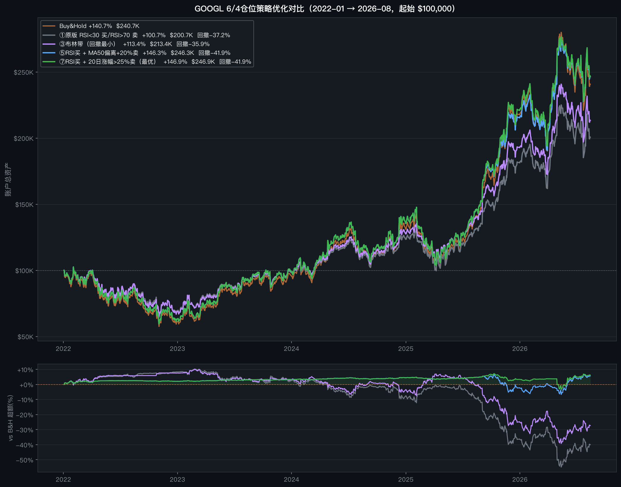
策略优化:7种方案对比(2026-08-17 补充)
对比结果
| 策略 | 最终资产 | 总收益 | 最大回撤 | 减仓次数 |
|---|---|---|---|---|
| ①原版 RSI>70 卖 | $200,670 | +100.7% | -37.2% | 65次 |
| ③布林带上轨卖 | $213,383 | +113.4% | -35.9% | 29次 |
| ②MA50偏离+12%卖 | $210,964 | +111.0% | -40.3% | 25次 |
| ⑥MA200趋势过滤 | $230,781 | +130.8% | -41.9% | 5次 |
| ④RSI买+MA50+15%卖 | $238,342 | +138.3% | -41.9% | 12次 |
| ⑤RSI买+MA50偏离+20%卖 ⭐ | $246,310 | +146.3% | -41.9% | 7次 |
| ⑦RSI买+20日涨幅>25%卖 | $246,923 | +146.9% | -41.9% | 3次 |
| 🟠 Buy & Hold(对照) | $240,681 | +140.7% | -43.6% | — |
三种减仓逻辑的本质区别
原版 RSI>70   → "涨了几天就减"    → 牛市里几乎每周触发 → 频繁踏空
布林带上轨    → "短期波动偏高就减"  → 稍好,但仍较频繁
**MA50 偏离+20% → "偏离均线够远才减"  → 真正的"相对高点" ← 推荐**
20日涨幅>25%  → "短期涨得太猛才减"  → 抓加速冲顶动作   ← 数据最优
⭐ 推荐策略:RSI 超卖加仓 + MA50 偏离减仓
核心改动:只改减仓触发条件,加仓逻辑不变。
把"RSI>70 就减"换成"价格超过 MA50 的 20% 才减"。
参数设定
| 参数 | 设定 | 说明 |
|---|---|---|
| 底仓 | 60% | 一次性买入,全程不动 |
| 浮动仓 | 40%(初始一半持股+一半现金) | 交易池 |
| 加仓触发 | RSI(14) < 30 | 超卖,下跌过度,加仓摊低 |
| 减仓触发 | 收盘价 > MA50 × 1.20 | 偏离50日均线20%,视为相对高点 |
| 每次加仓量 | 剩余浮动现金的 33% | 分批买入,不一次用完 |
| 每次减仓量 | 浮动持股的 40% | 分批卖出,保留仓位 |
| 冷却期 | 同方向 5 个交易日 | 防止同一波行情重复操作 |
为什么选 MA50 偏离 +20%,而不是 +15% 或涨幅>25%
| 方案 | 收益 | 减仓次数 | 问题 |
|---|---|---|---|
| MA50 +15% | +138.3% | 12次 | 阈值稍低,还是会在趋势中途触发 |
| MA50 +20% | +146.3% | 7次 | 均衡:抓到真正的高位,不乱动 |
| 20日涨幅>25% | +146.9% | 3次 | 数据略优,但震荡年里可能完全不触发,行为不稳定 |
MA50 偏离 20% 的直觉含义: 50日均线是过去2.5个月的平均成本,超过它20%意味着当前价格已经明显透支了近期买入者的预期。这是有均值基准的"相对高点",比 RSI 的"涨了几天"更有意义。
回测结论(2022-01 → 2026-08)
- 初始 $100,000 → 最终 $246,310(+146.3%)
- Buy & Hold 同期:$240,681(+140.7%)
- 策略跑赢 Buy & Hold $5,629,同时操作仅 43 次(加仓 34 + 减仓 7)
- 最大回撤 -41.9%(熊市防守略弱于原版,但牛市收益大幅补回)
核心教训
减仓触发器的选择决定策略成败。
- RSI>70 衡量的是"近期涨幅动能",在趋势股里长期偏高,不适合做减仓信号
- MA50 偏离度衡量的是"相对均值的高估程度",更接近"平均高点"的直觉
改完之后:减仓 65次 → 7次,收益 +100.7% → +146.3%,并跑赢 Buy & Hold。
数据来源
使用的库:yfinance
pip install yfinance
import yfinance as yf
df = yf.Ticker("GOOGL").history(start="2022-01-01", end="2026-08-15")
| 项目 | 说明 |
|---|---|
| 库名 | yfinance(Yahoo Finance 的非官方 Python 封装) |
| 数据提供方 | Yahoo Finance |
| 数据类型 | 日线 OHLCV(开盘/最高/最低/收盘/成交量) |
| 回测用字段 | 仅用 Close(每日收盘价) |
| 价格类型 | 复权后价格(Adjusted Close)——已自动反映拆股/分红 |
| 覆盖范围 | 全球主流股票/ETF/指数,历史数据可追溯 10~20 年 |
| 费用 | 完全免费,无需注册或 API Key |
重要:GOOGL 的 20:1 拆股
2022年7月18日,Alphabet 执行 20:1 股票拆分
拆分前:约 $2,800/股
拆分后:约 $140/股

yfinance 返回的历史数据已自动复权,
所以回测里 2022年1月的价格是 $143(已经是拆后调整价),
不是真实历史的 $2,860。

这不影响涨跌幅计算,但要注意:
从 yfinance 看到的 $83(2022年底部)
= 拆分前的 $1,660,是同一件事。
数据局限性
| 局限 | 说明 |
|---|---|
| 非官方接口 | Yahoo Finance 未公开 API,yfinance 是逆向封装,偶有数据中断或格式变化 |
| 收盘价 vs 实际成交 | 回测用收盘价买卖,现实中下单会有滑点(尤其大单) |
| 无盘前/盘后数据 | 财报后的跳空(GOOGL 常见)在收盘价层面被平滑掉了 |
| 历史数据可能微调 | Yahoo 偶尔会修正历史数据,重跑脚本结果可能有细微差异 |
数据验证方式
如果要核对某天价格是否正确:
1. 打开 finance.yahoo.com → 搜索 GOOGL
2. 点击 Historical Data → 设置日期范围
3. 与脚本输出的 Close 价格对比
或直接用代码验证:
import yfinance as yf
# 查某天的收盘价
df = yf.Ticker("GOOGL").history(start="2022-11-03", end="2022-11-04")
print(df[["Close"]])  # 应显示约 $82.7
脚本复现
依赖:pip install yfinance matplotlib
脚本一:回测计算(打印数据表)
import yfinance as yf
import pandas as pd
import numpy as np

# ─── 参数配置 ───────────────────────────────────────────
TOTAL_CAPITAL  = 100_000.0
BASE_RATIO     = 0.60        # 底仓比例
FLOAT_RATIO    = 0.40        # 浮动仓比例
RSI_BUY        = 30          # RSI 低于此值 → 加仓
RSI_SELL       = 70          # RSI 高于此值 → 减仓
BUY_FRAC       = 0.33        # 每次加仓:用剩余浮动现金的 33%
SELL_FRAC      = 0.40        # 每次减仓:卖出浮动股数的 40%
COOLDOWN       = 5           # 同方向冷却 5 个交易日
START          = "2022-01-03"
END            = "2026-08-15"

# ─── 数据获取 ────────────────────────────────────────────
df = yf.Ticker("GOOGL").history(start="2022-01-01", end=END)
df = df[["Open", "High", "Low", "Close"]].copy()
df.index = df.index.tz_localize(None)

# RSI-14
delta = df["Close"].diff()
gain  = delta.clip(lower=0).rolling(14).mean()
loss  = (-delta.clip(upper=0)).rolling(14).mean()
rs    = gain / loss.replace(0, np.nan)
df["RSI"] = 100 - 100 / (1 + rs)

df = df[df.index >= START]
open_price = df["Close"].iloc[0]

# ─── 初始状态 ────────────────────────────────────────────
base_shares  = (TOTAL_CAPITAL * BASE_RATIO) / open_price   # 底仓,一直持有
float_cash   = (TOTAL_CAPITAL * FLOAT_RATIO) * 0.5         # 浮动现金(初始 20000)
float_shares = (TOTAL_CAPITAL * FLOAT_RATIO) * 0.5 / open_price  # 浮动股(初始 20000 买入)

last_buy_day  = -999
last_sell_day = -999
trades        = []
equity_curve  = []

# ─── 逐日回测 ────────────────────────────────────────────
for i, (date, row) in enumerate(df.iterrows()):
    price = row["Close"]
    rsi   = row["RSI"]
    action = "—"

    if not np.isnan(rsi):
        # 加仓(低点)
        if rsi < RSI_BUY and float_cash > 1.0 and (i - last_buy_day) >= COOLDOWN:
            spend        = float_cash * BUY_FRAC
            float_shares += spend / price
            float_cash   -= spend
            last_buy_day  = i
            action        = "加仓↑"
            trades.append(dict(date=date, action=action, price=price,
                               rsi=rsi, float_cash=float_cash, float_shares=float_shares))

        # 减仓(高点)
        elif rsi > RSI_SELL and float_shares > 0.0001 and (i - last_sell_day) >= COOLDOWN:
            sold          = float_shares * SELL_FRAC
            float_cash   += sold * price
            float_shares -= sold
            last_sell_day = i
            action        = "减仓↓"
            trades.append(dict(date=date, action=action, price=price,
                               rsi=rsi, float_cash=float_cash, float_shares=float_shares))

    total_equity = (base_shares + float_shares) * price + float_cash
    equity_curve.append(dict(date=date, price=price, rsi=rsi,
                             total_equity=total_equity, action=action))

eq = pd.DataFrame(equity_curve).set_index("date")
tr = pd.DataFrame(trades) if trades else pd.DataFrame()

# ─── 结果输出 ────────────────────────────────────────────
final_price  = df["Close"].iloc[-1]
final_equity = (base_shares + float_shares) * final_price + float_cash
total_return = (final_equity - TOTAL_CAPITAL) / TOTAL_CAPITAL * 100
bnh_equity   = TOTAL_CAPITAL / open_price * final_price
bnh_return   = (bnh_equity - TOTAL_CAPITAL) / TOTAL_CAPITAL * 100

roll_max = eq["total_equity"].cummax()
max_dd   = ((eq["total_equity"] - roll_max) / roll_max * 100).min()
bnh_series  = TOTAL_CAPITAL / open_price * df["Close"]
bnh_max_dd  = ((bnh_series - bnh_series.cummax()) / bnh_series.cummax() * 100).min()

print(f"策略最终资产 : ${final_equity:,.2f}  ({total_return:+.1f}%)")
print(f"B&H 最终资产 : ${bnh_equity:,.2f}  ({bnh_return:+.1f}%)")
print(f"策略最大回撤 : {max_dd:.1f}%   B&H: {bnh_max_dd:.1f}%")
print(f"浮动仓操作   : 加仓 {(tr['action']=='加仓↑').sum()} 次 | 减仓 {(tr['action']=='减仓↓').sum()} 次")

# 逐年快照
checkpoints = ["2022-01-03","2022-06-30","2022-12-30",
               "2023-06-30","2023-12-29","2024-06-28",
               "2024-12-31","2025-06-30","2025-12-31","2026-08-14"]
for cp in checkpoints:
    rows = eq[eq.index >= cp]
    if rows.empty: continue
    r = rows.iloc[0]
    bv = TOTAL_CAPITAL / open_price * r["price"]
    print(f"{rows.index[0].date()}  策略 ${r['total_equity']:>10,.0f}  B&H ${bv:>10,.0f}")
脚本二:可视化图表(三图)
import yfinance as yf
import pandas as pd
import numpy as np
import matplotlib
matplotlib.use("Agg")
import matplotlib.pyplot as plt
import matplotlib.ticker as mtick

plt.rcParams["font.family"] = ["PingFang SC", "Heiti TC", "Arial Unicode MS", "DejaVu Sans"]
plt.rcParams["axes.unicode_minus"] = False

# ── 参数与脚本一保持一致 ──────────────────────────────────
TOTAL_CAPITAL  = 100_000.0
BASE_RATIO, FLOAT_RATIO = 0.60, 0.40
RSI_BUY, RSI_SELL       = 30, 70
BUY_FRAC, SELL_FRAC     = 0.33, 0.40
COOLDOWN = 5

df = yf.Ticker("GOOGL").history(start="2022-01-01", end="2026-08-15")
df = df[["Open","High","Low","Close"]].copy()
df.index = df.index.tz_localize(None)

delta = df["Close"].diff()
gain  = delta.clip(lower=0).rolling(14).mean()
loss  = (-delta.clip(upper=0)).rolling(14).mean()
df["RSI"] = 100 - 100 / (1 + gain / loss.replace(0, np.nan))
df = df[df.index >= "2022-01-03"]
open_price = df["Close"].iloc[0]

base_shares   = (TOTAL_CAPITAL * BASE_RATIO) / open_price
float_cash    = (TOTAL_CAPITAL * FLOAT_RATIO) * 0.5
float_shares  = (TOTAL_CAPITAL * FLOAT_RATIO) * 0.5 / open_price
last_buy_day  = last_sell_day = -999
buy_dates, buy_prices, sell_dates, sell_prices = [], [], [], []
equity_curve  = []

for i, (date, row) in enumerate(df.iterrows()):
    price, rsi = row["Close"], row["RSI"]
    if not np.isnan(rsi):
        if rsi < RSI_BUY and float_cash > 1.0 and (i - last_buy_day) >= COOLDOWN:
            float_shares += float_cash * BUY_FRAC / price
            float_cash   *= (1 - BUY_FRAC)
            last_buy_day  = i
            buy_dates.append(date); buy_prices.append(price)
        elif rsi > RSI_SELL and float_shares > 0.0001 and (i - last_sell_day) >= COOLDOWN:
            float_cash   += float_shares * SELL_FRAC * price
            float_shares *= (1 - SELL_FRAC)
            last_sell_day = i
            sell_dates.append(date); sell_prices.append(price)
    equity_curve.append((date, (base_shares + float_shares) * price + float_cash))

eq_df  = pd.DataFrame(equity_curve, columns=["date","equity"]).set_index("date")
bnh_df = (TOTAL_CAPITAL / open_price * df["Close"]).rename("bnh")

# ── 配色 ──────────────────────────────────────────────────
BLUE, GREEN, ORANGE, RED, PURPLE = "#58a6ff","#3fb950","#f0883e","#f85149","#bc8cff"
GRAY, BG, PANEL, BORDER = "#8b949e","#0d1117","#161b22","#30363d"

fig, axes = plt.subplots(3, 1, figsize=(14, 14),
                          gridspec_kw={"height_ratios": [3, 2, 1]})
fig.patch.set_facecolor(BG)
for ax in axes:
    ax.set_facecolor(PANEL)
    for sp in ax.spines.values(): sp.set_color(BORDER)
    ax.tick_params(colors=GRAY)

# Panel 1:资产曲线
ax1 = axes[0]
ax1.plot(eq_df.index, eq_df["equity"], color=BLUE,   lw=2,   label="策略(6底4浮)")
ax1.plot(bnh_df.index, bnh_df,         color=ORANGE, lw=1.5, label="Buy & Hold", alpha=0.8)
ax1.axhline(TOTAL_CAPITAL, color=GRAY, lw=0.8, ls="--", label="本金 $100K")
ax1.fill_between(eq_df.index, TOTAL_CAPITAL, eq_df["equity"],
                 where=eq_df["equity"] >= TOTAL_CAPITAL, alpha=0.12, color=GREEN)
ax1.fill_between(eq_df.index, TOTAL_CAPITAL, eq_df["equity"],
                 where=eq_df["equity"] < TOTAL_CAPITAL, alpha=0.12, color=RED)
ax1.set_title("GOOGL|6成底仓 + 4成浮动仓回测(2022-01 → 2026-08,起始 $100,000)",
              color="white", fontsize=13, pad=10, fontweight="bold")
ax1.set_ylabel("账户总资产", color=GRAY, fontsize=11)
ax1.yaxis.set_major_formatter(mtick.FuncFormatter(lambda x, _: f"${x/1000:.0f}K"))
leg = ax1.legend(framealpha=0.3, facecolor="#1c2128", fontsize=10)
for t in leg.get_texts(): t.set_color("white")
ax1.grid(axis="y", color=BORDER, lw=0.5)
final_eq, final_bnh = eq_df["equity"].iloc[-1], bnh_df.iloc[-1]
ax1.annotate(f"  策略 ${final_eq/1000:.1f}K (+{(final_eq/TOTAL_CAPITAL-1)*100:.1f}%)",
             xy=(eq_df.index[-1], final_eq), fontsize=10, color=BLUE, fontweight="bold")
ax1.annotate(f"  B&H ${final_bnh/1000:.1f}K (+{(final_bnh/TOTAL_CAPITAL-1)*100:.1f}%)",
             xy=(bnh_df.index[-1], final_bnh), fontsize=10, color=ORANGE, fontweight="bold")

# Panel 2:股价 + 交易点
ax2 = axes[1]
ax2.plot(df.index, df["Close"], color=GRAY, lw=1, label="GOOGL 收盘价")
ax2.scatter(buy_dates,  buy_prices,  color=GREEN, s=35, marker="^",
            label=f"加仓 ({len(buy_dates)}次)", edgecolors="#0d1117", linewidths=0.5)
ax2.scatter(sell_dates, sell_prices, color=RED,   s=35, marker="v",
            label=f"减仓 ({len(sell_dates)}次)", edgecolors="#0d1117", linewidths=0.5)
ax2.set_ylabel("GOOGL 股价 ($)", color=GRAY, fontsize=11)
ax2.yaxis.set_major_formatter(mtick.FuncFormatter(lambda x, _: f"${x:.0f}"))
leg2 = ax2.legend(framealpha=0.3, facecolor="#1c2128", fontsize=10, ncol=3)
for t in leg2.get_texts(): t.set_color("white")
ax2.grid(axis="y", color=BORDER, lw=0.5)

# Panel 3:RSI
ax3 = axes[2]
ax3.plot(df.index, df["RSI"], color=PURPLE, lw=1, label="RSI(14)")
ax3.axhline(70, color=RED,   lw=0.8, ls="--", label="超买 70 → 减仓")
ax3.axhline(30, color=GREEN, lw=0.8, ls="--", label="超卖 30 → 加仓")
ax3.fill_between(df.index, 70, df["RSI"].clip(upper=100), where=df["RSI"]>70, alpha=0.15, color=RED)
ax3.fill_between(df.index, df["RSI"].clip(lower=0), 30,  where=df["RSI"]<30, alpha=0.15, color=GREEN)
ax3.set_ylim(0, 100)
ax3.set_ylabel("RSI", color=GRAY, fontsize=11)
leg3 = ax3.legend(framealpha=0.3, facecolor="#1c2128", fontsize=9, ncol=3)
for t in leg3.get_texts(): t.set_color("white")
ax3.grid(axis="y", color=BORDER, lw=0.5)

fig.tight_layout(h_pad=2.5)
fig.savefig("googl_strategy_backtest.png", dpi=150, bbox_inches="tight", facecolor=BG)
print("图表已保存:googl_strategy_backtest.png")
See Also
- wiki/投资/core/决策框架/仓位管理-加仓与减仓.md — 加减仓的定性判断框架(信号 + 心理陷阱)
- wiki/投资/个人账户/持仓/GOOGL-Alphabet.md — 实际 GOOGL 持仓记录
- wiki/投资/core/心理/踏空痛苦与情绪驱动交易.md — 减仓后踏空的心理处理
- wiki/投资/震荡行情应对策略.md — 适合浮动仓策略的市场环境
- wiki/投资/core/关键指标/MACD背离-顶背离与底背离.md — 背离作为加仓信号的实证分析(底背离有效,顶背离在趋势股失效)
Sources
- 原始对话:
raw/投资/GOOGL-6底4浮RSI策略回测对话-20260817.md - 数据来源:yfinance GOOGL 历史收盘价(2022-01-03 ~ 2026-08-14)
- 回测日期:2026-08-17